Knowing how to access and exploit these features can be invaluable to your career and business. However, in addition to making your resume more enticing, it can also save you time and help you organize your life. Thus, in the following guide, we will explore twenty things to do in Excel that will make you an expert.
20 Things to Do in Excel That Will Make You an Expert
This guide will be a mixed bag of advanced and intermediate usage tips and tricks. We’ll cover operations such as pivot tables, functions, keyboard shortcuts, and more. Without further ado, here are the most useful tips, tricks, and hacks in Microsoft Excel.
1. Pivot Tables
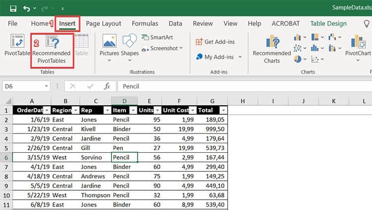
Pivot tables summarize your data for you. They are particularly useful when you’re working with large tables of data. They can save you from creating lots of summary calculations. The easiest way to create a pivot table using Microsoft Excel is:
Make sure that the table or spreadsheet you want to create the pivot table for is selectedClick on the Insert tabSelect Recommended Pivot Tables
From there, you’ll be able to select a few different options of how you might like to summarize your data. Selecting one of the recommended pivot tables will create a new spreadsheet with the pivot table inserted inside. If you plan to teach yourself how to use pivot tables, this is an excellent place to start. Once you understand how recommended pivot tables function, you can create your very own blank table. They also have content showing you how to arrange, slice and filter your pivot tables. If that isn’t enough, there is a wide variety of videos, books, and articles that can help you learn the intricacies of pivot tables.
2. Managing Duplicates
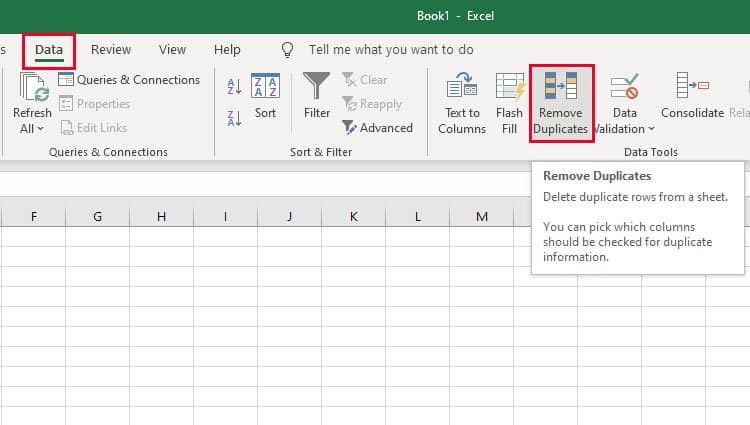
If you’re working with large sets of data, running into duplicate data is not uncommon. Fortunately, there are a couple of ways of eliminating duplicate data in Excel. You can either filter, use the Remove Duplicate data tool, or quick format for it. These are great alternatives to painstakingly and manually searching for duplicates yourself. Knowing how to manage duplicate data in Excel will make you look like a real expert.
3. Using VLOOKUP (Vertical Lookup)
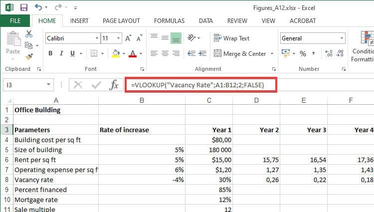
VLOOKUP is considered one of Excel’s most useful functions. If your data is organized into vertical columns, you can use the VLOOKUP function to search for a value in the first column of a sectioned data table. VLOOKUP will use the search value to return a corresponding value from another column. The VLOOKUP function takes four parameters:
Value: The search valueColumn_Range: The table or range of data columns you’re searching throughColumn_Number: The column number from which the corresponding value must be returned.Approximate_Match: A Boolean argument that instructs the function to either search for the exact match (0 or FALSE) or the approximate match (1 or TRUE). It’s an optional argument that is TRUE by default.
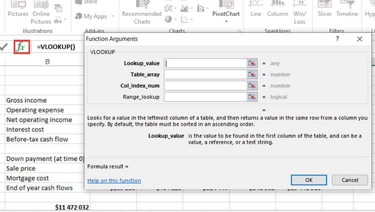
So the final function structure will look like this: VLOOKUP(Value; Column_Range; Column_Number; Approximate_Match) Again, VLOOKUP is particularly useful when you’re working with large sets of data. It can help you summarize or emphasize important figures in your spreadsheets. It’s even more accessible than ever. The latest versions of Excel provide you with a wizard to help you construct functions like VLOOKUP. All you need to do is click on the formulas button (fx) and select the VLOOKUP from the list. The wizard gives you an in-depth explanation of each required parameter. While typing out the function from scratch can make you look like a real Excel expert, using the Insert Function wizard is way easier. While this function is simple enough to understand and master, you can learn more about it from Microsoft’s official VLOOKUP tutorial.
4. Working with Multiple Excel Files
You can simultaneously open multiple Excel files in different Excel instances by selecting the files in your file explorer and pressing Enter on your keyboard. To quickly switch between Excel instances/files, simply press CTRL + TAB on your keyboard. This dazzling display of skill can make you look like some sort of Excel sorcerer to neophytes. Additionally, it can significantly increase your productivity.
5. Grouping and Ungrouping Worksheets
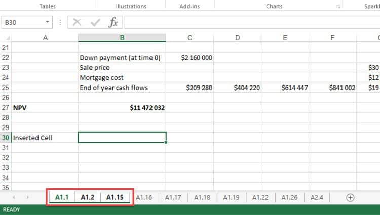
Grouping worksheets allows you to simultaneously edit multiple worksheets. To group your spreadsheets, do the following:
Hold the Ctrl button on your keyboard Select all the spreadsheets you want to groupRelease the Ctrl button
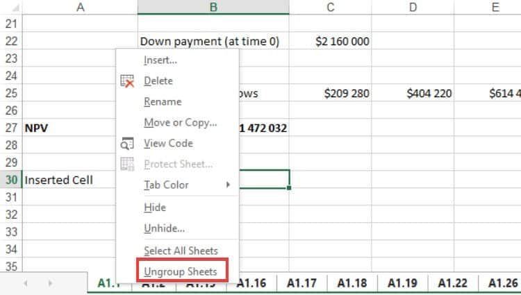
If you insert a value into any cell of any of the grouped spreadsheets, Excel will update all the spreadsheets with that value in the same cell. For instance, if you have three spreadsheets in a group and you update cell A30 of your first spreadsheet with the value “Insert Cell”, it will update cell A30 in the other spreadsheets in the group too. Grouping your worksheets is great for bulk editing. If you want to ungroup your spreadsheets, all you need to do is right-click on one of the spreadsheet tabs and select Ungroup Sheets from the context menu.
6. Using Freeze Panes
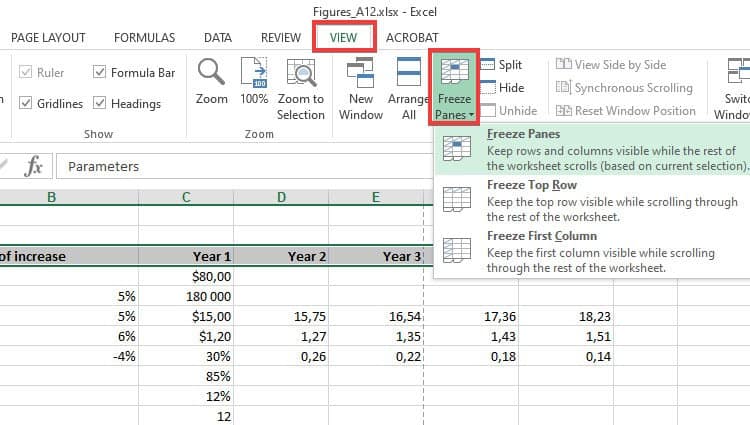
Excel has a freeze pane feature that allows you to freeze columns and rows. This makes it easier to compare and reference data. To access Freeze Panes:
Select cell/row underneath the row(s) you want to freezeClick on the VIEW tabClick on the Freeze Panes optionSelect Freeze Panes from the context menu
The row above your selected cell/row will be frozen as you scroll through your spreadsheet. Alternatively, you can select Freeze Top Row or Freeze First Column from the Freeze Panes menu. Freeze Top Row will freeze the first row for vertical scrolling, while Freeze First Column will freeze your first column for horizontal scrolling. To unfreeze your Panes, click on the Unfreeze Panes option from the Freeze Panes menu.
7. IF Function
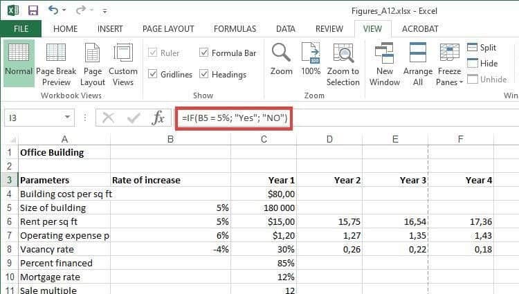
Excel’s IF function can make your data more dynamic. It’s a function that tells Excel to input or return a value if it meets a certain condition. It takes three parameters:
Logical_test: A test condition that can be validated as either true or falseValue_if_true: The value that Excel should use if the logical test is trueVaue_if_false: The value that Excel should use if the logical test is false
The logical test compares two values or cells using the equals (=), greater than (>), or the lesser than (<) symbols, e.g., = IF (C2>C3; “Yes”, “No”).
8. Using The Sum Function
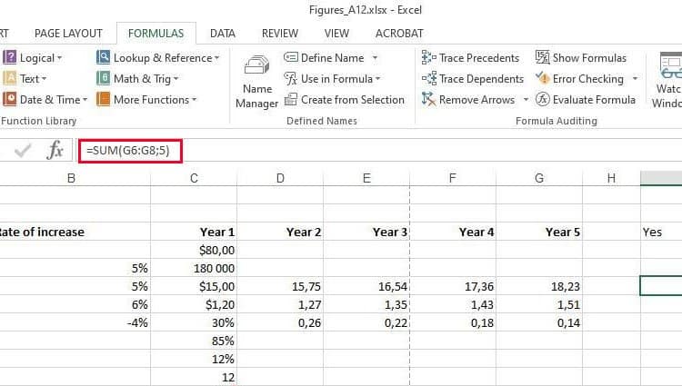
Excel allows you to perform a wide range of mathematical operations using one of its many functions. While you can perform advanced mathematical operations such as finding the cosine of an angle, it’s the simpler operations you may find useful. For instance, one of the most widely used math functions is the sum function. We use it to add numbers together. You can use cell indexes and/or actual numbers. The latest versions of Excel have an argument limit of 255 numbers. This means that you can have 255 terms. The syntax of the Sum function can look like this:
=Sum(1;2): Adds two simple numbers. The output will be 3.=Sum(A1;CB): Adds the contents of two cells together.=Sum(A1;2): Adds contents of a cell to a number. =Sum(A1:CB): Adds all the numbers in between (and including) these two indexes.=Sum(A1:CB;5): Adds all the numbers in a range of cells and adds an additional specified number to the sum.=Sum(A1:CB; G7:G1): Add all the numbers in two different cell index ranges.
These are only just a few of the variations. It’s a remarkably flexible function. If you want to appear even more impressive, you can use the SUMIF function, which combines the SUM function with the IF function.
9. Using The INDEX Function
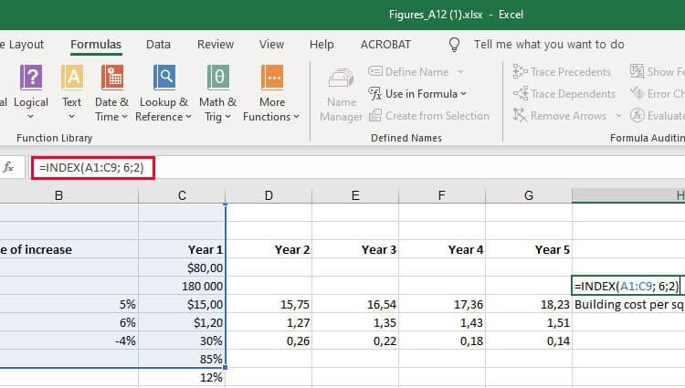
The INDEX function will return a value at the specified index within a table or a table section. It allows you to search for specific values in your spreadsheet. It comes in two forms:
Array Form – Takes an array for its first argument. The second argument is the row number, while the third is the column number. The array is constructed using the range of cells you want to search in your spreadsheet, i.e., A1:C20. The syntax of the function looks like this:=INDEX(array;row_num;col_num)=INDEX(A1:C20; 2; 3)
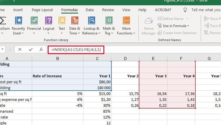
Reference Form – This takes a reference as its first argument. A reference allows you to input more than one range or a set of arrays. The second argument is the row number, and the third is the column number. The fourth allows you to select which array to search in. The syntax of the function looks like this:=INDEX((reference); row_num; col_num;area_num)e.g.=INDEX((A1:C9;D1:F8);2;3;1)
While the INDEX function is suited to simple searches, it can be used for advanced dynamic operations.
10. Using the MATCH Function
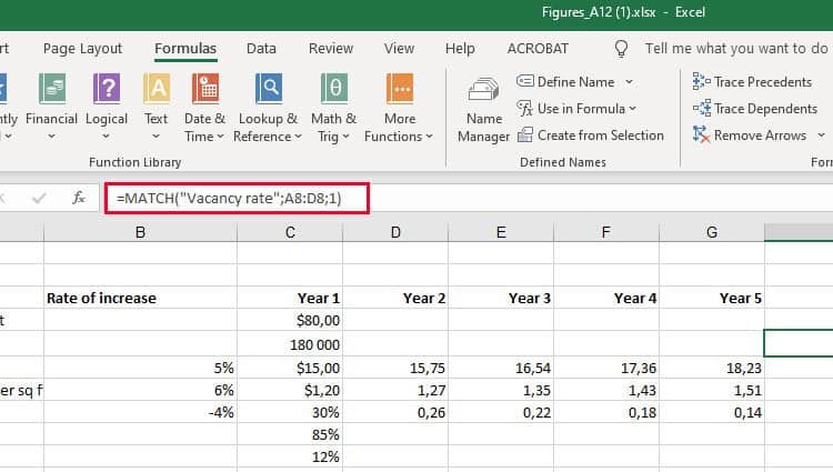
The MATCH function is another search function used to find the index of a value in a one-dimensional array/list (a table made up of one column or row). It consists of three arguments:
Search_Value: The value whose index you’re looking forArray_Range: The array or range of cells you want to search through – must consist of one column or row to work, i.e., A1:A9 or A1:E1Match_Type: An optional parameter that specifies if the function should find the exact match for the search value. It takes one of the following values: -1: Looks for the largest value that is less than or equal to the search value0: Looks for the exact match of the search value1: Looks for the smallest value that is greater than or equal to the search value
The syntax for the function looks like this: =MATCH(Search_Value; Array_Range;Match_Type)e.g.=MATCH(1; A1:A5;0)
11. Conditional Formatting
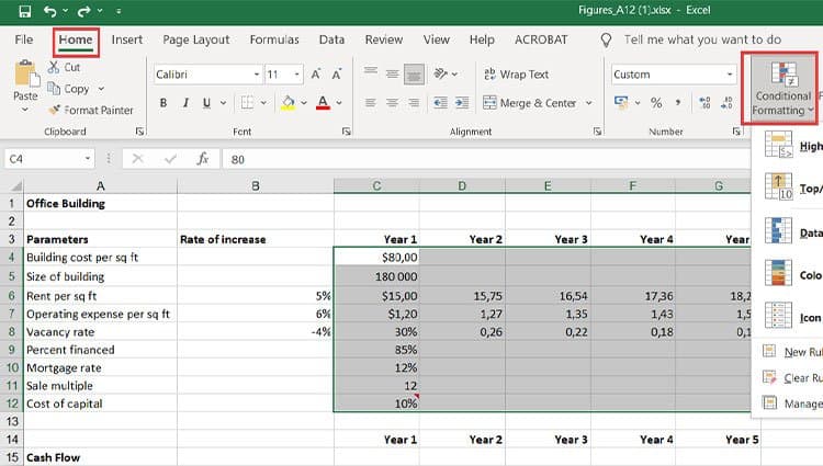
Much like charts, conditional formatting offers a way to visualize your data using color-coding that’s based on a cell’s value. To use conditional formatting, do the following:
Select all the cells you want formatted Click on the Home tabClick on Conditional Formatting
From there, you’ll be able to select which rules you’d like to instate for conditional formatting. You can even create your own custom rules.
12. Using Data Validation
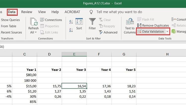
Data validation allows you to verify and ensure that your data is logical and fits certain parameters. If you’re working with text, it allows you to check if the text is spelled correctly. Excel’s Data Validation feature can be accessed by doing the following:
Select the cell or group of cells you want to perform data validation onClick on the Data tabClick on Data Validation
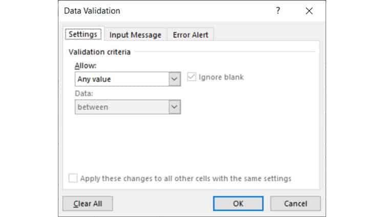
A dialog should pop up. It will allow you to set what type of values a cell allows. Additionally, it will allow you to set a range of acceptable values. You can also set an input message that displays itself when a cell is selected. The last tab in the data validation screen allows you to display an error alert when incorrect data is inserted into a cell.
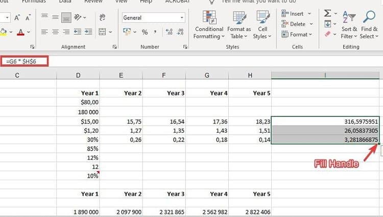
13. Using The Fill Handle to Copy Formulas
Excel allows you to fill in calculations across multiple cells. For instance, if you perform a calculation using cells from two different columns (but the same row), you can use the fill handle to copy the operation across multiple cells in the same column. To illustrate, if I perform a calculation in cell C1 where I multiply the contents of cell A1 by the contents of B1 (=A1B1) and drag the fill handle to cell C2, it will multiply the contents of cell A2 by B2 (=A2B2). While it’s a simple enough tool, knowing when or how to use it effectively can make you look like a real Excel expert.
14. Switching Between Relative, Absolute, and Mixed Cell References
In the previous entry, we spoke about using Excel’s fill handle. By default, the fill handle uses relative references. In other words, Excel will use the original calculation as a template and then infer its relative operands by looking at the position in the spreadsheet and looking at the original calculation’s operands. However, if you want more control over how Excel copies calculations across, you can use absolute cell references. This allows you to dictate some of the operands that get copied across. Thus, it enables you to copy a dynamic variable against a fixed value. For instance, you may want all the cells in column A to be multiplied by the contents of B1 (and only B1). To accomplish this, you’ll need to use a dollar sign ($) to lock the cell. Where you’re multiplying each cell in the A column by B1, the syntax of your calculation will look like this (=A1B$1). When you drag the fill handle, every affected cell in the column will multiply its contents by B1 (=A2B$1, =A3*B$1, etc.) Mastering this will bring you closer to becoming a real spreadsheet maestro.
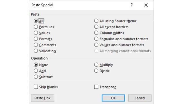
15. Using Paste Special
Excel allows you to control how you copy and paste data using its paste special feature. It allows you to copy and paste formatting, formulas, and values between cells. You can even use the paste special feature to perform a simple mathematical operation on copied data. To access the past special feature, do the following:
Copy your dataRight-click on the cell(s) you want to paste the data intoSelect Paste Special from the context menu
If you initiate the above steps correctly, you should be greeted by this dialog:
16. Transposing data in Excel
Microsoft Excel gives you a plethora of options to reposition or transpose data. You can transpose vertical (row) data into horizontal (column) data or vice versa using one of the following methods:
The Transpose functionThe Transpose Paste Special option
The easiest way would be to use the transpose paste option. However, it may seem far more impressive to master the Transpose function.
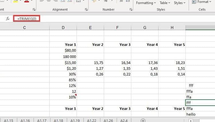
17. Using The TRIM Function
The TRIM function allows you to remove unwanted trailing and leading white spaces from Excel data. The Trim function only requires one argument (text). It will copy and input transposed data into a cell. The syntax of the trim function looks like this: =TRIM(Text)e.g.=TRIM(A1)=TRIM(“ hello world”) It’s a very simple function; however, if you work with a lot of text-based data, you may find it useful.
18. Using Macros
If you want to truly become an Excel expert, you’ll need to master Macros. Macros allow you to automate repetitive tasks in Excel by adding programming elements through Visual Basic code. You can even use Macros to extend some of Excel’s functionality. However, you don’t need programming experience to create basic Macros. Excel allows you to record repetitive actions, and it will write the code for you in the background. Covering Macros would take an entire article to explain in detail. Fortunately for you, there is a slew of content on the internet that will help you achieve a basic understanding of Macros.
19. Combining Functions
Excel allows you to combine multiple functions or formulas to expand their capabilities. For instance, while INDEX and MATCH are great search tools, they have limitations. To get around these limitations and initiate more advanced and dynamic searches, you can combine the two. For instance, you can use the MATCH function as the INDEX function’s row or column number i.e.=INDEX(Array_Range; MATCH(Search_Value; Array_Range;Match_Type);Column_Number)=INDEX(A1:C12;MATCH(“Size of building”;A1:A6);1) Once you learn how to master your most-used functions and formulas in Excel, you’ll get more comfortable with combining them. This is sure to make you look like an expert.
20. Keyboard Shortcuts
Using keyboard shortcuts in Excel is sure to make you look like an expert. However, not only does it make you look cool, it can save you time. We recommend you study and memorize an Excel keyboard shortcut cheat sheet. You can learn how to shift between tools, change your font, create a new spreadsheet, etc. All without having to use your mouse.
Conclusion
Microsoft Excel is a powerful business tool. One could say that it has the whole world’s financial system propped upon its shoulders. Becoming well-versed in Excel isn’t just a skill that will decorate your resume, but you can also use it to organize your life. In the above text, we explored 20 things you can do in Excel that will make you an expert. Do you have any tips or tricks of your own? Leave them down in the comment section below. As always, thank you for reading.